Musical TensorFlow, Part 2 - How to build an RNN-RBM for longer musical compositions in TensorFlow

Welcome to part 2 of the Musical TensorFlow series! In the last post, we built an RBM in TensorFlow for making short pieces of music. Today, we’re going to learn how to compose longer and more complex musical pieces with a more involved model: the RNN-RBM.

To warm you up, here’s an example of music that this network created:

Concepts

The RNN

A Recurrent Neural Network is a neural network architecture that can handle sequences of vectors. This makes it perfect for working with temporal data. For example, RNNs are excellent at tasks such as predicting the next word in a sentence or forecasting a time series.

In essence, an RNN is a sequence of neural network units where each unit \(u_t\) takes input from both \(u_{t-1}\) and data vector \(v_t\) and produces an output. Today most Recurrent Neural Networks utilize an architecture called Long Short Term Memory (LSTM), but for simplicity’s sake the RNN-RBM that we’ll make music with today uses a vanilla RNN.

If you haven’t worked with RNN’s before, Andrej Karpathy’s The Unreasonable Effectiveness of Recurrent Neural Networks is a must read. The RNN tutorial at wild-ml is great as well.

The RNN-RBM

The RNN-RBM was introduced in Modeling Temporal Dependencies in High-Dimensional Sequences: Application to Polyphonic Music Generation and Transcription (Boulanger-Lewandowski 2012). Like the RBM, the RNN-RBM is an unsupervised generative model. This means that the objective of the algorithm is to directly model the probability distribution of an unlabeled data set (in this case, music).

We can think of the RNN-RBM as a series of Restricted Boltzmann Machines whose parameters are determined by an RNN. As a reminder, the RBM is a neural network with 2 layers, the visible layer and the hidden layer. Each visible node is connected to each hidden node (and vice versa), but there are no visible-visible or hidden-hidden connections. The parameters of the RBM are the weight matrix \(W\) and the bias vectors \(bh\) and \(bv\).

The RBM:

We saw in the last post that an RBM is capable of modeling a complex and high dimensional probability distribution from which we can generate musical notes. In the RNN-RBM, the RNN hidden units communicate information about the chord being played or the mood of the song to the RBMs. This information conditions the RBM probability distributions, so that the network can model the way that notes change over the course of a song.

Model Architecture

One caveat: The RNN-RBM that I will describe below is not exactly identical to the one described in Boulanger-Lewandowski 2012. I’ve modified the model slightly to produce what I believe to be more pleasant music. All of my changes are superficial however, and the basic architecture of the model remains the same.

Also, for the rest of this post we will use \(u\) to represent the RNN hidden units, \(h\) to represent the RBM hidden units and \(v\) to represent the visible units (data).

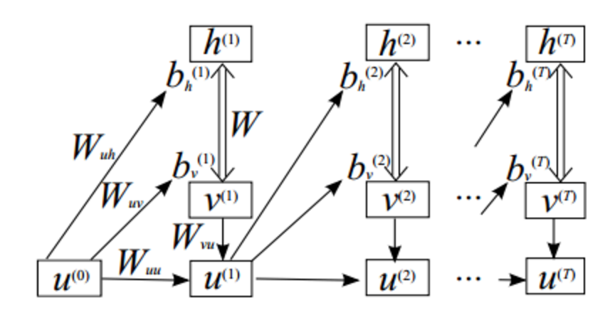
The architecture of the RNN-RBM is not tremendously complicated. Each RNN hidden unit is paired with an RBM. RNN hidden unit \(u_t\) takes input from data vector \(v_t\) (the note or notes at time t) as well as from RNN hidden unit \(u_{t-1}\). The outputs of hidden unit \(u_t\) are the parameters of \(RBM_{t+1}\), which takes as input data vector \(v_{t+1}\).

All of the RBMs share the same weight matrix, and only the hidden and visible bias vectors are determined by the outputs of \(u_t\). With this convention, the role of the RBM weight matrix is to specify a consistent prior on all of the RBM distributions (the general structure of music), and the role of the bias vectors is to communicate temporal information (the current state of the song).

Model Parameters

Note: Rather than adopt the naming convention from Boulanger-Lewandowski 2012, we use the much more sane naming convention from this deeplearning tutorial. The image below is also from this tutorial.

The parameters of the model are the following:

• \(W\), the weight matrix that is shared by all of the RBMs in the model
• \(W_{uh}\), the weight matrix that connects the RNN hidden units to the RBM hidden biases
• \(W_{uv}\), the weight matrix that connects the RNN hidden units to the RBM visible biases
• \(W_{vu}\), the weight matrix that connects the data vectors to the RNN hidden units
• \(W_{uu}\), the weight matrix that connects the the RNN hidden units to each other
• \(b_u\), the bias vector for the RNN hidden unit connections
• \(b_v\), the bias vector for the RNN hidden unit to RBM visible bias connections. This vector serves as the template for all of the \(b_v^{t}\) vectors
• \(b_h\), the bias vector for the RNN hidden unit to RBM hidden bias connections. This vector serves as the template for all of the \(b_h^{t}\) vectors

Training

Note: Before training the RNN-RBM, it is helpful to initialize \(W\), \(bh\), and \(bv\) by training an RBM on the dataset, according to the procedure specified in the previous post.

To train the RNN-RBM, we repeat the following procedure:

1. In the first step we communicate the RNN’s knowledge about the current state of the song to the RBM. We use the RNN-to-RBM weight and bias matrices and the state of RNN hidden unit \(u_{t-1}\) to determine the bias vectors \(b_{v}^{t}\) and \(b_{h}^{t}\) for \(RBM_t\).
   • \[b_{h}^{t} = b_{h} + u_{t-1}W_{uh}\]
   • \[b_{v}^{t} = b_{v} + u_{t-1}W_{uv}\]
2. In the second step we create a few musical notes with the RBM. We initialize \(RBM_t\) with \(v_{t}\) and perform a single iteration of Gibbs Sampling to sample \(v_{t}^{*}\) from \(RBM_t\). As a reminder, Gibbs sampling is a procedure for drawing a sample from the probability distribution specified by an RBM. You can see the previous post for a more thorough description of Gibbs sampling.
   • \(h_i \backsim \sigma (W^{T}v_t + b_{h}^{t})_i\).
   • \(v_{t_{i}}^{*} \backsim \sigma (Wh + b_{v}^{t})_i\).
3. In the third step we compare the notes that we generated with the actual notes in the song at time \(t\). To do this we compute the contrastive divergence estimation of the negative log likelihood of \(v_t\) with respect to \(RBM_t\). Then, we backpropagate this loss through the network to compute the gradients of the network parameters and update the network weights and biases. In practice, TensorFlow will handle the backpropagation and update steps.
   • We compute this loss function by taking the difference between the free energies of \(v_t\) and \(v_{t}^{*}\).
     • \[loss = F(v_{t}) - F(v_{t}^{*}) \simeq -log(P(v_t))\]
4. In the fourth step we use the new information to update the RNN’s internal representation of the state of the song. We use \(v_t\), the state of RNN hidden unit \(u_{t-1}\) and the weight and bias matrices of the RNN to determine the state of RNN hidden unit \(u_{t}\). In the below equation, we can substitute \(\sigma\) for other non-linearities, such as \(tanh\).
   • \[u_{t} = \sigma(b_{u} + v_{t}W_{vu} + u_{t-1}W_{uu})\]

Generation

To use the trained network to generate a sequence, we initialize an empty generated_music array and repeat the same steps as above, with some simple changes. We replace steps 2 and 3 with:

• Initialize the visible state of \(RBM_t\) (with \(v_{t-1}^{*}\) or zeros) and perform \(k\) steps of Gibbs Sampling to generate \(v_{t}^{*}\)
• Add \(v_{t}^{*}\) to the generated_music array

We also replace the \(v_{t}\) in the equation in step 4 with \(v_{t}^{*}\).

Data and Music

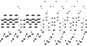
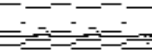
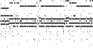
The data format is identical to the data format in the previous post - that is, midi piano rolls. Below are some piano rolls of human-generated and RNN-RBM generated songs:

A folk song from the Nottingham database:

A portion of the song “Fix You” by Coldplay.

An RNN-RBM song:

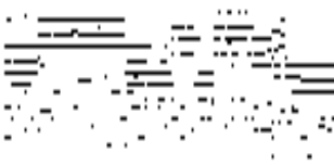
Another RNN-RBM song:

Here is some music that was produced by training the RNN-RBM on a small dataset of pop music midi files.

In Boulanger-Lewandowski 2012, each RBM only generates one timestep, but I’ve found that allowing each RBM to generate 5 or more timesteps actually produces more interesting music. You can see the specifics in the code below.

Code

All of the RNN-RBM code is in this directory. If you’re not interested in going through the code and just want to make music, you can follow the instructions in the README.md.

Here is what you need to look at if you are interested in understanding and possibly improving on the code:

• weight_initializations.py When you run this file from the command line, it instantiates the parameters of the RNN-RBM and pretrains the RBM parameters by using Contrastive Divergence.
• RBM.py This file contains all of the logic for building and training the RBMs. This is very similar to the RBM code from the previous post, but it has been refactored to fit into the RNN-RBM model. The get_cd_update function runs an iteration of contrastive divergence to train the RBM during weight initialization, and the get_free_energy_cost function computes the loss function during training.
• rnn_rbm.py This file contains the logic to build, train, and generate music with the RNN-RBM. The rnnrbm function returns the parameters of the model and the generate function, which we call to generate music.
• rnn_rbm_train.py When you run this file from the command line, it builds an RNN-RBM, sets up logic to compute gradients and update the weights of the model, spins up a TensorFlow session, and runs through the data, training the model.
• rnn_rbm_generate.py When you run this file from the command line, it builds an RNN-RBM, spins up a TensorFlow session, loads the weights of the RNN-RBM from the saved_weights_path that you supply, and generates music in the form of midi files.

Extensions

The basic RNN-RBM can generate music that sounds nice, but it struggles to produce anything with temporal structure beyond a few chords. This motivates some extensions to the model to better capture temporal dependencies. For example, the authors implement Hessian-Free optimization, an algorithm for efficiently performing 2nd order optimization. Another tool that is very useful for representing long term dependencies is the LSTM cell. It’s reasonable to suspect that converting the RNN cells to LSTM cells would improve the model’s ability to represent longer term patterns in the song or sequence, such as in this paper by Lyu et al.

Another way to increase the modelling power of the algorithm is to replace the RBM with a different model. The authors of Boulanger-Lewandowski 2012 replace the RBM with a neural autoregressive distribution estimator (NADE), which is a similar algorithm that models the data with a tractable distribution. Since the NADE is tractable, it doesn’t suffer from the gradient-approximation errors that contrastive divergence introduces. You can see here that the music generated by the RNN-NADE shows more local structure than the music generated by the RNN-RBM.

We can also replace the RBM with a Deep Belief Network, which is an unsupervised neural network architecture formed from multiple RBMs stacked on top of one another. Unlike RBMs, DBNs can take advantage of their multiple layers to form hierarchical representations of data. In this later paper from Vohra et al, the authors combine DBNs and LSTMs to model high dimensional temporal sequences and generate music that shows more complexity than the music generated by an RNN-RBM.

Extensions

Thanks for joining me today to talk about making music in TensorFlow! If you enjoyed seeing how neural networks can learn how to be creative, you may enjoy some of these other incredible architecures:

• The neural style algorithm is one of the most breathtaking algorithms for computational art ever created. The algorithm repaints a photograph or image in the style of a painting. The algorithm works by training a convolutional neural network to maximize both the generated image’s pixel to pixel coherence with the photograph and the texture similarity of the generated image and the painting.

  

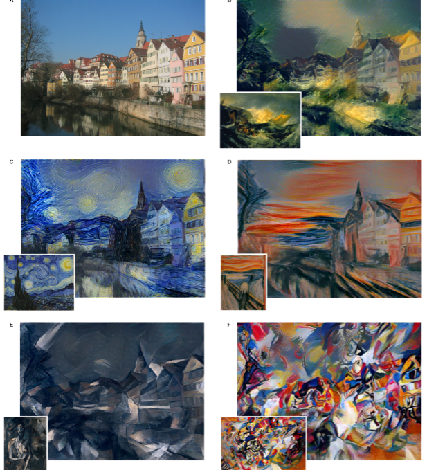
  Here is a TensorFlow implementation and a torch implementation of the algorithm

• The DRAW neural network is a recurrent neural network architecture for generating images. The network adds a sequencial component to image generation by sliding a virtual “pen” to “draw” an image. You can find an accessible description of the paper here.

• The DCGAN architecture is one of the most exciting new neural network architectures. This algorithm involves training 2 “adversarial” neural networks to battle each other. One network generates images, and the other network tries to distinguish the generated images from real images. This architecture has shown incredible success in generating pictures of bedrooms and faces that look almost real.