Generative models are awesome. TensorFlow is awesome. Music is awesome. In this post, we’re going to use TensorFlow to build a generative model that can create snippets of music.
I’m going to assume that you have a pretty good understanding of neural networks and backpropagation and are at least a little bit familiar with TensorFlow. If you haven’t used TensorFlow before, the tutorials are a good place to start.
Concepts
Generative Models
Generative Models specify a probability distribution over a dataset of input vectors. For an unsupervised task, we form a model for \(P(x)\), where \(x\) is an input vector. For a supervised task, we form a model for \(P(x \vert y)\), where \(y\) is the label for \(x\). Like discriminative models, most generative models can be used for classification tasks. To perform classification with a generative model, we leverage the fact that if we know \(P(X \vert Y)\) and \(P(Y)\), we can use bayes rule to estimate \(P(Y \vert X)\).
Some good resources for learning about generative models include:
-
A nice and simple visual description of machine learning and the difference between generative and discriminative models.
-
An excellent description of some popular generative algorithms. My personal favorite resource. Honestly all of the notes for Andrew Ng’s class are solid gold.
-
A heavily referenced paper that compares linear discriminative and generative models. The moral of the story is that generative models tend to be better at classification when data is sparse, and discriminative classifiers are better when data is plentiful. Also written by Andrew Ng.
Unlike discriminative models, we can also use generative models to create synthetic data by directly sampling from the modelled probability distributions. I think that this is pretty sweet, and I’m going to prove it to you. But first, let’s talk about RBMs.
The Restricted Boltzman Machine
If you have never encountered RBMs before, they can be a little complex. I’m going to quickly review the details below, but if you want understand them more thoroughly, the following resources may be helpful:
-
This article contains a good, very visual description of RBMs. Also includes a DL4J implementation.
-
This post is a relatively in-depth description of RBMs, starting from a description of Energy-Based models. Also includes an implementation in Theano.
-
Here is a pretty intuitive description of RBMs as binary factor analysis. This article also includes a description of the classic movie rating RBM example.
RBM Architecture
The RBM is a neural network with 2 layers, the visible layer and the hidden layer. Each visible node is connected to each hidden node (and vice versa), but there are no visible-visible or hidden-hidden connections (the RBM is a complete bipartite graph). Since there are only 2 layers, we can fully describe a trained RBM with 3 parameters:
- The weight matrix \(W\):
- \(W\) has size \(n_{visible}\ x\ n_{hidden}\). \(W_{ij}\) is the weight of the connection between visible node \(i\) and hidden node \(j\).
- The bias vector \(bv\):
- \(bv\) is a vector with \(n_{visible}\) elements. Element \(i\) is the bias for the \(i^{th}\) visible node.
- The bias vector bh:
- \(bh\) is a vector with n_hidden elements. Element \(j\) is the bias for the \(j^{th}\) hidden node.
\(n_{visible}\) is the number of features in the input vectors. \(n_{hidden}\) is the size of the hidden layer.

In this image we remove most of the edges for clarity.
RBM Sampling
Unlike most of the neural networks that you’ve probably seen before, RBMs are generative models that directly model the probability distribution of data and can be used for data augmentation and reconstruction. To sample from an RBM, we perform an algorithm known as Gibbs sampling. Essentially, this algorithm works like this:
-
Initialize the visible nodes. You can initialize them randomly, or you can set them equal to an input example.
-
Repeat the following process for \(k\) steps, or until convergence:
- Propagate the values of the visible nodes forward, and then sample the new values of the hidden nodes.
- That is, randomly set the values of each \(h_i\) to be \(1\) with probability \(\sigma (W^{T}v + bh)_i\).
- Propagate the values of the hidden nodes back to the visible nodes, and sample the new values of the visible nodes.
- That is, randomly set the values of each \(v_i\) to be 1 with probability \(\sigma (Wh + bv)_i\).
- Propagate the values of the visible nodes forward, and then sample the new values of the hidden nodes.
At the end of the algorithm, the visible nodes will store the value of the sample.
RBM Training
Remember that an RBM describes a probability distribution. When we train an RBM, our goal is to find the values for its parameters that maximize the likelihood of our data being drawn from that distribution.
To do that, we use a very simple strategy:
- Initialize the visible nodes with some vector \(x\) from our dataset
- Sample \(\tilde{x}\) from the probability distribution by using Gibbs sampling
- Look at the difference between the \(\tilde{x}\) and \(x\)
- Move the weight matrix and bias vectors in a direction that minimizes this difference
The equations are straightforward:
\[W = W + lr(x^{T}h(x) - \tilde{x}^{T}h(\tilde{x}))\\ bh = bh + lr(h(x) - h(\tilde{x}))\\ bv = bv + lr(x - \tilde{x})\]- \(x_t\) is the inital vector
- \(\tilde{x}\) is the sample of x drawn from the probability distribution
- \(lr\) is the learning rate
- \(h\) is the function that takes in the values of the visible nodes and returns a sample of the hidden nodes (see step 1 of the Gibbs sampling algorithm above)
This technique is known as Contrastive Divergence. If you want to learn more about CD, you can check out this excellent derivation.
Implementation
Data
In this tutorial we are going to use our RBM to generate short sequences of music. Our training data will be around a hundred midi files of popular songs. Midi is a format that directly encodes musical notes - you can think of midi files as sheet music for computers. You can play midi files or convert them to mp3 by using a tool such as GarageBand. Midi files encode events that a synthesizer would need to know about, such as Note-on, Note-off, Tempo changes, etc. For our purposes, we are interested in getting the following information from our midi files:
- Which note is played
- When the note is pressed
- When the note is released
We can encode each song with a binary matrix with the following structure:
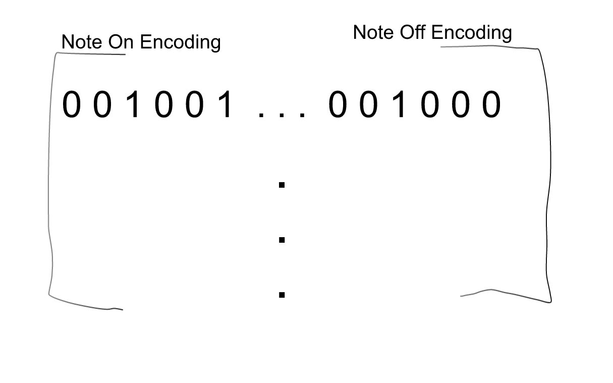
The first n columns (where n is the number of notes that we want to represent) encode note-on events. The next n columns represent note-off events. So if element \(M_{ij}\) is 1 (where \(j< n\)), then at timestep \(i\), note \(j\) is played. If element \(M_{i (n+j)}\) is 1, then at timestep \(i\), note \(j\) is released.
In the above encoding, each timestep is a single training example. If we reshape the matrix to concatenate multiple rows together, then we can represent multiple timesteps in a single data vector.
Converting midi files to and from these binary matrices is relatively simple, but there are a number of annoying edge cases. All of the code for reading and writing midi files is in the midi_manipulation.py file, which is heavily based on Daniel Johnson’s midi manipulation code. Midi files aren’t really the point of this post, but if you want to know more, the following libraries are pretty useful:
- python-midi contains fundamental tools for reading and writing midi files in python
- music21 is a more advanced (and complicated) midi library
Code
Now let’s get coding! In order for the code below to work, you need to put it in a directory with the following files:
For your convenience, all of the code is in this repository. Just follow the instructions in the README.md.
import numpy as np
import pandas as pd
import msgpack
import glob
import tensorflow as tf
from tensorflow.python.ops import control_flow_ops
from tqdm import tqdm

###################################################
# In order for this code to work, you need to place this file in the same
# directory as the midi_manipulation.py file and the Pop_Music_Midi directory

import midi_manipulation

def get_songs(path):
    files = glob.glob('{}/*.mid*'.format(path))
    songs = []
    for f in tqdm(files):
        try:
            song = np.array(midi_manipulation.midiToNoteStateMatrix(f))
            if np.array(song).shape[0] > 50:
                songs.append(song)
        except Exception as e:
            raise e
    return songs

songs = get_songs('Pop_Music_Midi') #These songs have already been converted from midi to msgpack
print "{} songs processed".format(len(songs))
###################################################

### HyperParameters
# First, let's take a look at the hyperparameters of our model:

lowest_note = 24 #the index of the lowest note on the piano roll
highest_note = 102 #the index of the highest note on the piano roll
note_range = highest_note-lowest_note #the note range

num_timesteps  = 15 #This is the number of timesteps that we will create at a time
n_visible      = 2*note_range*num_timesteps #This is the size of the visible layer.
n_hidden       = 50 #This is the size of the hidden layer

num_epochs = 200 #The number of training epochs that we are going to run. For each epoch we go through the entire data set.
batch_size = 100 #The number of training examples that we are going to send through the RBM at a time.
lr         = tf.constant(0.005, tf.float32) #The learning rate of our model

### Variables:
# Next, let's look at the variables we're going to use:

x  = tf.placeholder(tf.float32, [None, n_visible], name="x") #The placeholder variable that holds our data
W  = tf.Variable(tf.random_normal([n_visible, n_hidden], 0.01), name="W") #The weight matrix that stores the edge weights
bh = tf.Variable(tf.zeros([1, n_hidden],  tf.float32, name="bh")) #The bias vector for the hidden layer
bv = tf.Variable(tf.zeros([1, n_visible],  tf.float32, name="bv")) #The bias vector for the visible layer


#### Helper functions.

#This function lets us easily sample from a vector of probabilities
def sample(probs):
    #Takes in a vector of probabilities, and returns a random vector of 0s and 1s sampled from the input vector
    return tf.floor(probs + tf.random_uniform(tf.shape(probs), 0, 1))

#This function runs the gibbs chain. We will call this function in two places:
#    - When we define the training update step
#    - When we sample our music segments from the trained RBM
def gibbs_sample(k):
    #Runs a k-step gibbs chain to sample from the probability distribution of the RBM defined by W, bh, bv
    def gibbs_step(count, k, xk):
        #Runs a single gibbs step. The visible values are initialized to xk
        hk = sample(tf.sigmoid(tf.matmul(xk, W) + bh)) #Propagate the visible values to sample the hidden values
        xk = sample(tf.sigmoid(tf.matmul(hk, tf.transpose(W)) + bv)) #Propagate the hidden values to sample the visible values
        return count+1, k, xk

    #Run gibbs steps for k iterations
    ct = tf.constant(0) #counter
    [_, _, x_sample] = control_flow_ops.While(lambda count, num_iter, *args: count < num_iter,
                                         gibbs_step, [ct, tf.constant(k), x], 1, False)
    #This is not strictly necessary in this implementation, but if you want to adapt this code to use one of TensorFlow's
    #optimizers, you need this in order to stop tensorflow from propagating gradients back through the gibbs step
    x_sample = tf.stop_gradient(x_sample)
    return x_sample

### Training Update Code
# Now we implement the contrastive divergence algorithm. First, we get the samples of x and h from the probability distribution
#The sample of x
x_sample = gibbs_sample(1)
#The sample of the hidden nodes, starting from the visible state of x
h = sample(tf.sigmoid(tf.matmul(x, W) + bh))
#The sample of the hidden nodes, starting from the visible state of x_sample
h_sample = sample(tf.sigmoid(tf.matmul(x_sample, W) + bh))

#Next, we update the values of W, bh, and bv, based on the difference between the samples that we drew and the original values
size_bt = tf.cast(tf.shape(x)[0], tf.float32)
W_adder  = tf.mul(lr/size_bt, tf.sub(tf.matmul(tf.transpose(x), h), tf.matmul(tf.transpose(x_sample), h_sample)))
bv_adder = tf.mul(lr/size_bt, tf.reduce_sum(tf.sub(x, x_sample), 0, True))
bh_adder = tf.mul(lr/size_bt, tf.reduce_sum(tf.sub(h, h_sample), 0, True))
#When we do sess.run(updt), TensorFlow will run all 3 update steps
updt = [W.assign_add(W_adder), bv.assign_add(bv_adder), bh.assign_add(bh_adder)]


### Run the graph!
# Now it's time to start a session and run the graph!

with tf.Session() as sess:
    #First, we train the model
    #initialize the variables of the model
    init = tf.initialize_all_variables()
    sess.run(init)
    #Run through all of the training data num_epochs times
    for epoch in tqdm(range(num_epochs)):
        for song in songs:
            #The songs are stored in a time x notes format. The size of each song is timesteps_in_song x 2*note_range
            #Here we reshape the songs so that each training example is a vector with num_timesteps x 2*note_range elements
            song = np.array(song)
            song = song[:np.floor(song.shape[0]/num_timesteps)*num_timesteps]
            song = np.reshape(song, [song.shape[0]/num_timesteps, song.shape[1]*num_timesteps])
            #Train the RBM on batch_size examples at a time
            for i in range(1, len(song), batch_size):
                tr_x = song[i:i+batch_size]
                sess.run(updt, feed_dict={x: tr_x})

    #Now the model is fully trained, so let's make some music!
    #Run a gibbs chain where the visible nodes are initialized to 0
    sample = gibbs_sample(1).eval(session=sess, feed_dict={x: np.zeros((10, n_visible))})
    for i in range(sample.shape[0]):
        if not any(sample[i,:]):
            continue
        #Here we reshape the vector to be time x notes, and then save the vector as a midi file
        S = np.reshape(sample[i,:], (num_timesteps, 2*note_range))
        midi_manipulation.noteStateMatrixToMidi(S, "generated_chord_{}".format(i))
Music Samples
By altering the num_timesteps variable in the above code, we can make sequences of music of different lengths. Since each additional timestep increases the dimensionality of the vectors we are inputting to the model, we are limited to sequences of only a few seconds. In my next post, I’ll show how we can adapt this model to generate longer sequences of music.
15 timesteps
10 timesteps
5 timesteps
Wrap Up
I hoped you enjoyed this post about RBMs in TensorFlow! RBMs have a plethora of applications that are more useful than generating short sequences of music, but their real power comes when we build them into more complex models. For example, we can form Deep Belief Networks by stacking RBMs into multiple layers. Training a DBN is simple - we greedily train each RBM, and pass the mean activations of each trained RBM as input to the next layer. Unlike RBMs, DBNs can take advantage of deep learning to learn hierarchical features of the data.
In the next post, we’re going to talk about a different model that builds on the RBM - the RNN-RBM. This model is a sequence of RBMs, where the parameters of each RBM is determined by an Recurrent Neural Network. This architecture can model temporal dependencies, and we will use the model to generate much longer, more complex, and better-sounding musical pieces.