Bayesian Attack Detection for Smarter SOCs

No generative AI here - just good old-fashioned statistics.

This post introduces Bayesian networks: visual models that connect the clues you see to the threats you care about. Instead of drowning in isolated alerts, a Bayesian network lets your SOC update its belief about an attack as new evidence arrives. We’ll minimize heavy math and focus on how to learn, build, and use Bayesian Networks in practice.

Thinking like a Bayesian

Suppose you notice a signal - like a login from a new device - that almost never happens during normal activity, but is much more common when an account is actually compromised. Intuitively, if you see this rare event, you should strongly suspect an attack.

Here’s a simple numeric example: if odd login times happen once in every 1,000 benign logins, but once in every 10 attacks, then seeing one makes compromise 100× more likely. That’s the core of Bayesian reasoning: weigh how surprising a signal is under normal conditions versus attack conditions.

Bayesian networks help by letting you encode multiple such relationships as probabilities: you specify how likely a signal is in benign versus attack scenarios, and the network does the math to update your belief automatically. This makes it possible to combine many such clues-even if each is imperfect-into a coherent, quantitative assessment of risk.

The Signal-Combination Problem

Modern SOCs deal with thousands of alerts daily. Analysts validate each alert by gathering context: Was MFA disabled? Was it a new device? Was the login at a weird time?

Analysts are already doing a form of Bayesian updating: starting with a low prior belief that a real incident is in progress and adjusting that belief as new clues appear. Bayesian networks formalize this, allowing us to combine multiple signals without over-counting.

Mini-case: imagine an attacker disables MFA, logs in from a new device, and attempts a privileged action. Each individual clue is noisy, but together the BN may raise P(Account Compromise) from 2% to 80% - and flag the case for immediate escalation.

Bayesian Reasoning in Plain English

Start with a prior belief: Real incidents are rare, so P(attack) is low.
Weight evidence by how surprising it is: If a signal like login from NordVPN is rare in benign conditions but common in real attacks, it’s a strong clue.
Combine multiple pieces of evidence: Bayesian networks only connect clues when they’re dependent. This avoids double-counting correlated signals like Impossible Travel and New Device.

Building a Bayesian Detection Network

A Bayesian network (BN) is a directed graph of variables (signals or outcomes). Edges capture conditional dependencies. Here’s a structured way to build one:

Pick the outcome Example: Account Compromise.
List your key signals 6–10 strong indicators you already track: Impossible Travel, MFA Disabled, New Device, Privileged Action, Critical Asset Access.
Draw arrows for dependencies Example: Impossible Travel → New Device, MFA Disabled → Account Compromise.
Assign probabilities Use incident history, baselines, or expert judgment. Imperfect numbers are fine - the network learns as you validate cases.
Update with evidence As new alerts fire, the BN computes P(attack | signals) and explains which clues had the most impact.

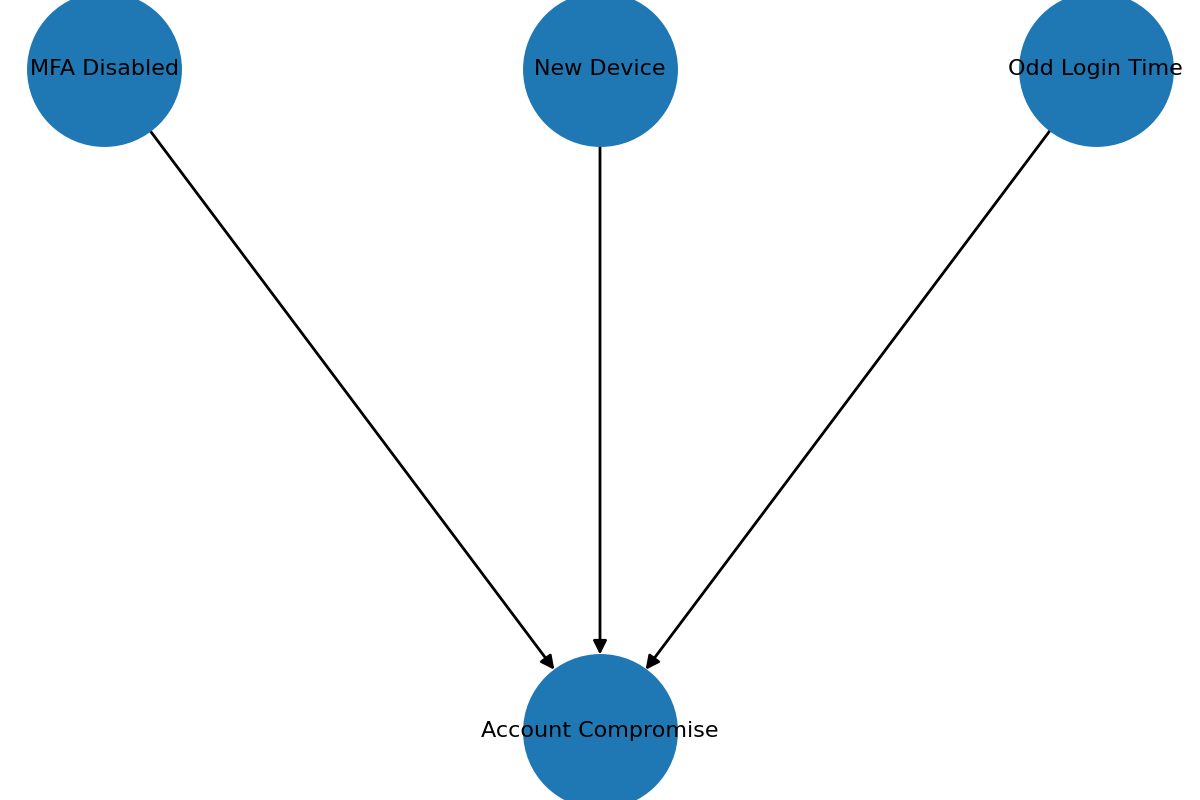
Example

Here’s a simple example network:

account compromise

And here it is in Python

from pgmpy.models import DiscreteBayesianNetwork
from pgmpy.factors.discrete import TabularCPD
from pgmpy.inference import VariableElimination

# The structure of the network (three independent signals in this case)
model = DiscreteBayesianNetwork([
    ("MFA_Disabled", "Account_Compromise"),
    ("New_Device", "Account_Compromise"),
    ("Odd_Login_Time", "Account_Compromise")
])

# The prior probabilities of the signals
cpd_mfa = TabularCPD("MFA_Disabled", 2, [[0.95], [0.05]])
cpd_device = TabularCPD("New_Device", 2, [[0.9], [0.1]])
cpd_time = TabularCPD("Odd_Login_Time", 2, [[0.85], [0.15]])

# The conditional probability of an attack given each signal
cpd_attack = TabularCPD(
    "Account_Compromise", 2,
    [[0.999, 0.98, 0.97, 0.9, 0.95, 0.7, 0.6, 0.2],   # Not compromised
     [0.001, 0.02, 0.03, 0.1, 0.05, 0.3, 0.4, 0.8]],  # Compromised
    evidence=["MFA_Disabled", "New_Device", "Odd_Login_Time"],
    evidence_card=[2, 2, 2]
)

Learning the Network From Data

Now once you have some data you can use it to update your model:

import pandas as pd
from pgmpy.estimators import BayesianEstimator

# Your data
df = pd.DataFrame([
    [0,0,0,0],[0,1,0,0],[0,1,1,1],[1,0,0,0],[1,1,1,1],
    [0,0,1,0],[0,1,1,0],[0,0,0,0],[1,0,1,1],[0,1,0,0],
    [0,0,1,0],[1,1,0,1],[0,0,0,0],[0,1,1,1],[0,0,0,0],
    [1,0,0,0],[0,1,0,0],[0,0,1,0],[1,1,1,1],[0,0,0,0],
], columns=["MFA_Disabled", "New_Device", "Odd_Login_Time", "Account_Compromise"])

# Build the model
model.add_cpds(cpd_mfa, cpd_device, cpd_time, cpd_attack)
est = BayesianEstimator(model, df)
cpd_mfa_up    = est.estimate_cpd("MFA_Disabled", prior_type="BDeu", equivalent_sample_size=10)
cpd_device_up = est.estimate_cpd("New_Device",    prior_type="BDeu", equivalent_sample_size=10)
cpd_time_up   = est.estimate_cpd("Odd_Login_Time",prior_type="BDeu", equivalent_sample_size=10)

# Update the model with the new data
model.remove_cpds(cpd_mfa, cpd_device, cpd_time)
model.add_cpds(cpd_mfa_up, cpd_device_up, cpd_time_up, cpd_attack)

Pitfalls and Guardrails

Base-rate blindness Priors matter. Rare but benign events can look malicious without proper baselines. Mitigation: calibrate priors using historical data or baselining tools.
Double counting Connect correlated signals explicitly to avoid inflating probabilities. Mitigation: model dependencies with edges (e.g., New Device → Impossible Travel).
Missing data Bayesian inference handles missingness gracefully, but you should document assumptions and clarify how absent signals are interpreted. Mitigation: explicitly decide whether “missing” means neutral, suspicious, or benign.
Explainability Keep networks simple enough for analysts to interpret. Complexity should never outweigh clarity. Mitigation: prioritize interpretability over marginal gains in accuracy.

Takeaway

Bayesian networks give SOCs a transparent, mathematically principled way to combine signals. They scale intuition, explain their reasoning, and learn over time.

Start small with just a few signals, and then expand as you get comfortable.