Introduction
Many prediction problems can be framed as “given the knowledge that this sample belongs to categories \(A,B,C,\cdots,D\), predict something about this sample.” As a concrete example, suppose we would like to use linear regression to predict the value of a transaction based on a small set of categorical features \((f_1, f_2, \cdots, f_n)\). These could involve things like the identity of the vendor, the time of day, etc. There are many ways that we could represent these features.
One-Hot Encodings
One way that we could design our model to consume these features would be to use a one-hot encoding of each categorical feature. That is, if we have \(n\) total features such that the \(i\)th feature \(f_i\) is a categorical feature with \(n_i\) possible values, then the dimensionality of our total feature vector would be \(\sum_{i=1\cdots n} n_i\). Each element of this feature vector would be either \(0\) or \(1\) depending on the categories that the sample belongs to.
Another strategy would be to cross our categorical features before we one-hot encode them. When we cross the categorical features \(f_i, f_j\) we create a new categorical feature \((f_i,f_j)\) whose value is the tuple of the values of \(f_i\) and \(f_j\). This tuple has \(n_i*n_j\) possible values. In the extreme case we could cross all of our categorical features together to form the single crossed feature \((f_1,f_2,\cdots,f_n)\). This feature has \(\prod_{i=1\cdots n} n_i\) possible values, so its one-hot encoding is a vector with \(\prod_{i=1\cdots n} n_i\) elements.
To start, assume that there is only a single categorical feature with \(n_0\) distinct values. In this case the two strategies are identical. For a sample that belongs to category \(j \in [0, 1, \cdots, n_0]\) the model prediction will simply be \(\theta_j\). That is, our model functions as simply a lookup table. If the transaction values of the samples in category \(j\) follow a Gaussian distribution then the value of \(\theta_j\) that minimizes our model’s mean square error will be the average transaction value of all samples in category \(j\).
Next, assume that there are \(n\) categorical features, and the \(i\)th categorical feature has \(n_i\) distinct values and consider a sample that belongs to categories \((k_1, k_2, \cdots, k_n)\).
- In the case with no feature crosses, the prediction of our model on a sample that belongs to categories \((k_1, k_2, \cdots, k_n)\) will be \(\sum_{i=1\cdots n} \theta_{\sum_{j=1\cdots i} n_i + k_i}\). That is, the prediction is the sum of \(n\) non-zero numbers, each corresponding to one of the categories that sample belongs to. In this case our model functions as a linear combination of lookup tables.
- In the extreme feature crossing case where we cross all of the features, the prediction of our model will be \(\theta_{k_1, k_2, \cdots, k_n}\). Once again our model is simply a lookup table, and if we assume a Gaussian distribution on transactions the value \(\theta_{k_1, k_2, \cdots, k_n}\) will be the average transaction value for all samples that belonging to each of the categories \((k_1, k_2, \cdots, k_n)\) in our training data.
Aggregations
Another way to design our model would be to compute the average transaction value for each of the categories that the sample might belong to, and to use these averages as the features. Like in the one-hot case we have the choice of whether to cross these categories before computing these averages. Note that these kinds of features are sometimes referred to as “counting features” or “aggregate features.” Note that in practice we would probably standardize these features before feeding them to the linear model.
In the case that we don’t cross any of the features before aggregating the feature vector for a sample that belongs to the categories \((k_1, k_2, \cdots, k_n)\) will be an \(n\)-element vector whose \(i\)th component is the average transaction value for all samples that belong to category \(k_i\) of categorical feature \(f_i\). In the extreme case that we cross all of the categories before aggregating the feature vector for a sample that belongs to the categories \((k_1, k_2, \cdots, k_n)\) will be a single number: the average transaction value for all samples that belong to the categories \((k_1, k_2, \cdots, k_n)\).
Cross Features and Data
Utilizing either the one-hot encoding or aggregation strategies requires making the decision of whether to cross our features before feeding them to our model. In both strategies fully crossing all features is optimal in the case that we have infinite training data. This enables the model to treat each collection of categories independently and represent relationships between them like “midnight transactions tend to be small, transactions at bars tend to be small, but midnight transactions at bars tend to be large.”
However, the less training data that we have, the less likely that we will have enough examples in each combination of categories to generate a good prediction. A common strategy to handle this in both the one-hot and aggregate cases is to include both the crossed and uncrossed features in the model. Then the model can learn weights on these features that represents their predictive power. We can think of the model strategy as being something like: when presented with a user that belongs to the categories \((k_1, k_2, \cdots, k_n)\), check the averages of each category and each combination of categories, weight each average by how much we trust it, and then sum these weighted averages.
Infrastructure Burden and Data Distribution Shift
The infrastructure burden on realtime responsiveness lives in different places for the one-hot features and aggregate features. Fetching and serving features is extremely easy in the one-hot encoding model. For any transaction, the only thing we need to feed to the model are the categories of that transaction. In contrast, the aggregate model expects to be served averages for each of the categories that a transaction belongs to. Serving features to this model requires looking these averages up at request time, and these averages need to be kept updated in order for the model to produce good results. Furthermore, backtesting a new aggregation strategy on old data requires simulating how the aggregation would have been performed up until that data sample was observed, which can be quite complex if the aggregation code and model training code live in different services or are written in different languages.
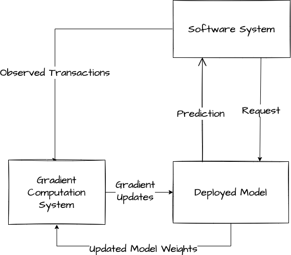
However, enabling a one-hot model to respond to data distribution shift requires a major infrastructure investment. To see this, suppose that we have already deployed our model to production. Suppose also that one of the categories in our transaction prediction model is the vendor identity, and that one of the vendors in our pool decides to roll out a new line of fancy coffee that substantially increases the average transaction amount. In the case where our model consumes the features as a one-hot encoding, our model will produce incorrect predictions until it is retrained with data that includes the new fancy coffee transactions. That is, in order for our modeling pipeline to respond to data distribution shift we need for the new data samples to reach our database, get transformed into a gradient update, and be applied to our production model. Generally the best way to equip our model to adapt to this kind of distribution shift in realtime is to train the model itself online. That is, derive gradient updates from each new transaction that we observe and apply them to our deployed model on the fly. This kind of online training system can be quite complex to maintain in production.
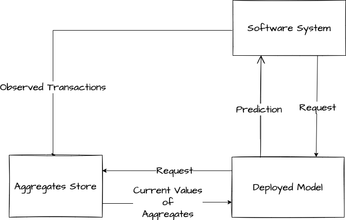
In constrast, consider the case where our model consumes the features as category-stratified aggregates. In this case our model will produce incorrect predictions only until the new fancy coffee transactions are incorporated into the aggregate values that are fed into the model as features. We can get nearly instant adaptation to data distribution shift if our aggregates are engineered to update in near-realtime. This could be done through either realtime re-computation from the backing data store or posting updates to a running average stored in memory.
Conclusion
Although we assume that our model is a linear regression in this post, the ideas we discuss are very general. In practice most large machine learning systems consume categorical signals as a combination of one-hot encoded features and running averages. Signals that are unlikely to change too quickly are often best encoded one-hot, whereas signals for which realtime responsiveness is paramount are ideally represented as running aggregates.