There are 2 closely related quantities in statistics - correlation (often referred to as \(R\)) and the coefficient of determination (often referred to as \(R^2\)). Today we’ll explore the nature of the relationship between \(R\) and \(R^2\), go over some common use cases for each statistic and address some misconceptions.
Correlation
The correlation of 2 random variables \(A\) and \(B\) is the strength of the linear relationship between them. If A and B are positively correlated, then the probability of a large value of \(B\) increases when we observe a large value of \(A\), and vice versa. If we are observing samples of \(A\) and \(B\) over time, then we can say that a positive correlation between \(A\) and \(B\) means that \(A\) and \(B\) tend to rise and fall together.
Covariance and Correlation
In order to understand correlation, we need to discuss covariance. The variance of a random variable \(A\) is \(var(A) = E[(A - E[A])^2]\), where \(E[A]\) is the expected value of A. The variance is a measure of the spread or dispersion of a random variable around its expected value. Note that variance is not a scale invariant feature - if we have some random variable measured in miles and we convert it to kilometers, then the variance of the random variable will increase.
Covariance is the extension of variance to the 2-variable case - it is a measure of the joint variability of 2 random variables. The covariance of \(A\) and \(B\) is \(Cov(A,B) = E[(A - E[A])(B - E[B])]\). Note that like variance, covariance is not scale invariant. If the variance of \(A\) or \(B\) increases, then \(Cov(A,B)\) increases as well. Since the covariance is the product of the dispersions of \(A\) and \(B\) from the mean, \(Cov(A,B)\) is largest when \(A\) and \(B\) move together, and is negative when they move opposite from each other. These are the same properties that correlation exhibits, and this is not a coincidence. The correlation of \(A\) and \(B\) is the covariance of \(A\) and \(B\) normalized by their variances. That is, \(Corr(A,B) = Cov(A,B)/\sqrt{var(A)var(B)}\).
Correlation Features and Bugs
There are a few important features of correlation that we should talk about:
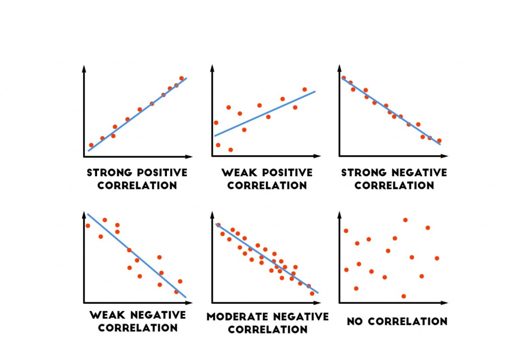
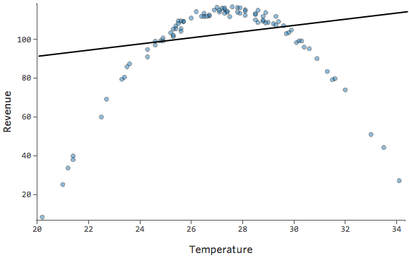
- The correlation between \(A\) and \(B\) is only a measure of the strength of the linear relationship between \(A\) and \(B\). Two random variables can be perfectly related, to the point where one is a deterministic function of the other, but still have zero correlation if that function is non-linear. In the following graph the X and Y variables are clearly dependent, but because their relationship is strongly non-linear, their correlation is close to zero.
- There is a simple geometric interpretation of correlation. In the following analysis I will assume that \(A\) and \(B\) have expected value 0 in order to make the math easier, but the results still hold even if this is not the case. Let’s say we take n samples of \(A\) and n samples of \(B\), and then form vectors \(v_{a}\) and \(v_{b}\) from the samples of \(A\) and \(B\). The empirical variance of \(A\) is then \(E[(A - E[A])^2] = E[(A)^2] = v_{a} \cdot v_{a} = \Vert v_{a} \Vert ^2\). Similarly, the empirical covariance of \(A\) and \(B\) is \(E[(A - E[A])(B - E[B])] = E[(A)(B)] = v_{a} \cdot v_{b}\). Therefore, since (by the definition of dot product) \(v_{a} \cdot v_{b} = (\Vert v_{a}\Vert)(\Vert v_{b}\Vert)(cos(v_{a}, v_{b}))\), the cosine of the angle between \(v_{a}\) and \(v_{b}\) is equivalent to the correlation of \(A\) and \(B\).

It’s worthwhile to note that this property is useful for reasoning about the bounds of correlation between a set of vectors. If vector \(A\) is correlated with vector \(B\) and vector \(B\) is correlated with another vector \(C\), there are geometric restrictions to the set of possible correlations between \(A\) and \(C\).
- Correlation is invariant to scaling and shift. That is, \(Corr(A,B) = Corr(cA + x, B)\). This property is a double edged sword: correlation can detect a relationship between variables on very different scales, but it can be insensitive to changes in the distributions of variables if those changes only affect scale and shift.
Using Correlation as a Performance Metric
Lets say you are performing a regression task (regression in general, not just linear regression). You have some response variable \(y\), some predictor variables \(X\), and you’re designing a function \(f\) such that \(f(X)\) approximates \(y\). You want to check how closely \(f(X)\) approximates \(y\). Can you use correlation? There are definitely some benefits to this - correlation is on the easy to reason about scale of -1 to 1, and it generally becomes closer to 1 as \(f(X)\) looks more like \(y\). There are also some glaring negatives - the scale of \(f(X)\) can be wildly different from that of \(y\) and correlation can still be large. Lets look at some more useful metrics for evaluating regression performance.
Mean Square Error
The Mean Square Error (MSE) of our regression is \((1/n)\sum{(y - f(X))^2}\). Does this look familiar? It should - if we have \(f(X) = E[y]\) for all \(X\), then this becomes \((1/n)\sum{(y - E[y])^2} = E[(y - E[y])^2] = var(y)\). So any function \(f(X)\) that does better than just predicting the mean should have lower MSE than the variance of \(y\).
Lets say that we’re trying to estimate the weight of an object, and \(y\) is measured in kg. Then the MSE of our regression will be measured in kg^2, which isn’t all that easy to reason about. For this reason we often also look at the Root Mean Square Error (RMSE), defined as the square root of the MSE. The RMSE of our regression is an estimate of how wrong our regression is on average.
The Coefficient of Determination
Like everything in statistics, there are a number of problems with MSE and RMSE. For example, their scales depend on the units of \(y\). This means that we can’t easily compare the performance of models across related tasks. For this reason, it seems that we would benefit from defining a unit-invariant metric that scales the MSE by the variance of \(y\). This metric, \(1 - MSE/var(y)\), is the coefficient of determination, \(R^2\).
So lets get a sense of the range of \(R^2\). It’s pretty clear that a model that always predicts the mean of \(y\) will have an MSE equal to \(var(y)\) and an \(R^2\) of 0. A model that is worse than the mean-prediction model (such as a model that always predicts a number other than the mean) will have a negative \(R^2\). A model that predicts \(y\) perfectly will have an MSE of 0 and an \(R^2\) of 1.
R…squared?
So what is the relationship between \(R\) and \(R^2\)? It’s pretty clear that computing the coefficient of determination is not always as simple as squaring the correlation, since \(R^2\) can be less than 0. However, there are certain conditions under which the squared correlation is equivalent to the coefficient of determination.
For example, let’s consider the case where we fit a linear regression to some dataset \(X, y\) and compute \(R\) and \(R^2\) between \(y\) and the predicted values \(f(X)\) (i.e. the training/in-sample \(R\) and \(R^2\)). In this case there are a few nice properties. First, if we use an intercept term we can guarantee that \(\bar{f} = \bar{y}\) (i.e. the means of the predicted values and the true values are equal). Next, we can decompose the sum of the squared errors of \(y\) (\(SS_{tot}\), basically \((n)(var(y))\)) into a component that is “explained” by the regression and a component that is “not explained” by the regression. The “explained” component is the sum of the squared deviances of the regression values from the mean (\(SS_{reg} = (f_i - \bar{y})^2\)), and the not explained component is the sum of the squared residual values (\(SS_{res} = (f_i - y_i)^2\)). Therefore \(\sum{(y_i - \bar{y})^2} = \sum{(f_i - \bar{y})^2} + \sum{(f_i - y_i)^2}\) and \(SS_{tot} = SS_{res} + SS_{reg}\). You can check out the proof of this here.
So why is this fact useful? Well \(R^2 = 1 - MSE/var(y) = 1 - SS_{res}/SS_{tot} = 1 - (SS_{tot} - SS_{reg})/SS_{tot} = 1 - 1 + SS_{reg}/SS_{tot} = SS_{reg}/SS_{tot}\). Therefore, under these conditions \(R^2\) is equal to the ratio of the variance explained by the regression to the total variance (which is a fact you may have heard out of context).
Now we can prove that the square of the correlation coefficient is equivalent to the ratio of explained variance to the total variance. Let’s start with the definition of correlation:
\(R = cov(y, f)/\sqrt{var(y)var(f)} =\)
\(\sum{(y_i - \bar{y})(f_i - \bar{y})}/\sqrt{\sum{(y_i - \bar{y})^2}\sum{(f_i - \bar{y})^2}} =\)
\((\sum{(y_i - f_i)(f_i - \bar{y}) + (f_i - \bar{y})}) / \sqrt{\sum{(y_i - \bar{y})^2}\sum{(f_i - \bar{y})^2}} =\)
\(\sum{(f_i - \bar{y})^2} / \sqrt{\sum{y_i - \bar{y})^2}\sum{(f_i - \bar{y})^2}} =\)
\(\sqrt{\sum{(f_i - \bar{y})^2} / \sum{(y_i - \bar{y})^2}}\)
Which is exactly the square root of \(SS_{reg}/SS_{tot}\). Note that on the third step we use the fact that the sum of the in sample residuals for a linear regression is zero.
Let’s take a step back. We’ve shown that when we are comparing the predictions of a linear regression model to the truth values over the training data, then the square of the correlation is equivalent to the coefficient of determination. What about over the test data? Well, in the case where the features are completely uncorrelated with the response values, the linear regression will end up predicting the mean of the training data. If this is different from the mean of the test data, then the \(R^2\) over the test data will be negative.
In fact, the square of the correlation coefficient is generally equal to the coefficient of determination whenever there is no scaling or shifting of \(f\) that can improve the fit of \(f\) to the data. For this reason the differential between the square of the correlation coefficient and the coefficient of determination is a representation of how poorly scaled or improperly shifted the predictions \(f\) are with respect to \(y\).
Conclusion
Both \(R\), MSE/RMSE and \(R^2\) are useful metrics in a variety of situations. Generally, \(R\) is useful for picking up on the linear relationship between variables, MSE/RMSE are useful for quantifying regression performance and \(R^2\) is a convenient rescaling of MSE that is unit invariant. And remember, when somebody quotes an \(R^2\) number for you, make sure to ask whether it’s \(R^2\) or the square of \(R\).