Introduction
The Mapper algorithm is a useful tool for identifying patterns in a large dataset by generating a graph summary. We can describe the Mapper algorithm as constructing a discrete approximation of the Reeb graph:
Suppose we have a manifold \(\mathbf{X}\) equipped with a distance metric \(d_{\mathbf{X}}\) (such as a submanifold of \(\mathbb{R}^d\) equipped with Euclidean distance) and a continuous function \(f: \mathbf{X} \rightarrow \mathbb{R}\). Define the equivalence relation \(\sim_{f}\) over the points in \(\mathbf{X}\) such that \(x \sim_{f} x'\) if and only if there exists some \(y\) in the image of \(f\) such that \(x\) and \(x'\) belong to the same connected component of \(f^{-1}(y)\). The Reeb graph \(R_{f}(\mathbf{X})\) is the quotient space \(\mathbf{X} / \sim_{f}\) endowed with the quotient topology. Intuitively, the Reeb graph contracts connected components of level sets of \(f\) into single points.
Now suppose we have a set of points \(X \subset \mathbf{X}\) that we assume have been drawn according to some probability measure \(\mu_{\mathbf{X}}\) over \(\mathbf{X}\). Suppose also that we have a computable function \(f_{X}: X \rightarrow \mathbb{R}\) that approximates \(f: \mathbf{X} \rightarrow \mathbb{R}\). The function \(f_{X}\) may depend on the exact sample \(X\) from \(\mathbf{X}\). For example, if \(f(x)\) is the probability density at \(x\), then \(f_{X}\) could be a density estimator such as the distance from a point in \(X\) to its \(k\)-nearest neighbor in \(X\). The Mapper algorithm uses \((X, d_{\mathbf{X}})\) and \(f_{X}\) to construct an approximation of the Reeb graph \(R_{f}(\mathbf{X})\):
- Select a collection \(\mathcal{C}\) of open intervals of length \(r\) that cover \(f_{X}(X)\) such that the intersection of any three intervals in \(\mathcal{C}\) is empty and the overlap between any two consecutive intervals is a fixed constant.
- For each interval \(I \in \mathcal{C}\), apply a clustering algorithm (such as K-Means or Agglomerative Clustering) to form a partition of \(f_{X}^{-1}(I) \subseteq X\). Note that the clusters across each \(f_{X}^{-1}(I)\) form an overlapping cover of \(X\).
- Create an \(n\)-simplex for each collection of \(n\) clusters in this overlapping cover that have non-empty intersection. This creates a simplicial complex. We refer to the \(1\)-skeleton of this complex as the Mapper graph.
One challenge with using Mapper in practice is that the algorithm may generate substantially different graphs for different datasets drawn from the same distribution. In order to use Mapper to make confident conclusions about a data-generating distribution, it is important to have a strong intuition about the algorithm’s stability under resampling. In this post we perform a case study to explore the empirical convergence properties of Mapper. We build bootstrap samples of different sizes from two real-world datasets, Fashion-MNIST and Wikipedia+Gigaword 5, and construct Mapper graphs from these samples. We then explore the relationship between the sample size and the distributions of structural invariants of these Mapper graphs. The code for these experiments is hosted here.
Experiments
We focus on the following structural invariants of Mapper graphs \(G\):
- Number of Connected Components: If we view \(G\) as a simplicial complex, its number of connected components is equivalent to the \(0^{th}\) Betti number of the complex.
- Cardinality of Cycle Basis: The cardinality of the cycle basis of \(G\) is the minimum size of a set of cycles that span the cycle space of \(G\). If we view \(G\) as a simplicial complex, the cardinality of the cycle basis is equivalent to the \(1^{st}\) Betti number of the complex.
- Graph Density: The density of an undirected graph \(G\) with \(k\) nodes and \(h\) edges is \(\frac{2h}{k(k-1)}\). As \(n\) increases, we would expect both \(k\) and \(h\) to increase as well, and the density will track the relative rates of increase.
- Estrada Index: The Estrada index of an undirected graph \(G\) whose adjacency matrix has eigenvalues \(\lambda_1, \lambda_2, ..., \lambda_n\) is \(\sum_{i=1}^n e^{\lambda_i}\). The Estrada index measures the centrality of \(G\), or the degree to which each node in \(G\) participates in the subgraphs of \(G\).
We explore how stable these graph invariants are when we run Mapper with AgglomerativeClustering. We use the \(k\)-nearest neighbor filter function, and we run this algorithm with a variety of \(k\) and resolution values over the following real-world datasets:
-
Fashion-MNIST: This dataset includes \(70,000\) unique \(28 \times 28\) images of clothing that fall into \(9\) classes. To simplify the dataset and reduce the distance between points in the same class we apply the supervised UMAP algorithm to reduce the dimensionality from \(784\) to \(50\).
-
Word Vectors from Wikipedia+Gigaword 5: This dataset contains \(400,000\) unique \(50\) dimensional gloVe embeddings of words.
We compute the stability of these graph invariants via the bootstrap procedure. For each dataset, we choose an \(n\)-element sample (with replacement) from the dataset, run Mapper over this sample to build an undirected graph \(G \in \mathcal{G}\), and then compute each invariant. We repeat this process \(100\) times for each value of \(n\) and assess the relationship between \(n\) and each graph invariant’s coefficient of variation, or the ratio of its empirical mean and standard deviation.
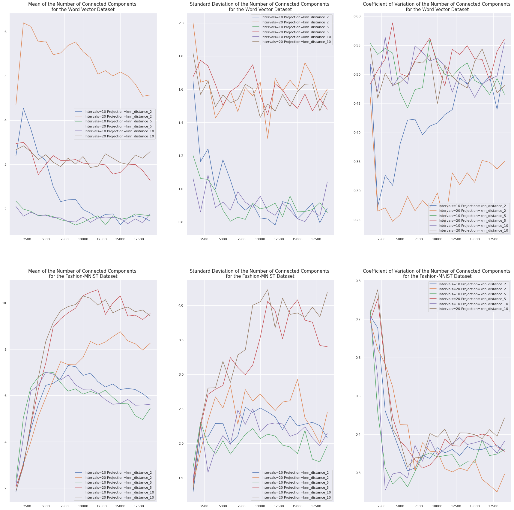
Number of Connected Components
Each data point in Fashion-MNIST falls into one of \(9\) distinct classes, and the number of connected components seems to converge to around \(9\) as the number of points increases. This is especially true when the resolution (number of intervals) is larger. The coefficient of variation therefore drops very quickly as the sample size increases.
In contrast, we don’t see any such effect in the Word Vector dataset, and the coefficient of variation of this graph invariant does not consistently decrease as the sample size increases. This is probably because the categories into which words fall tend to overlap, especially across language.
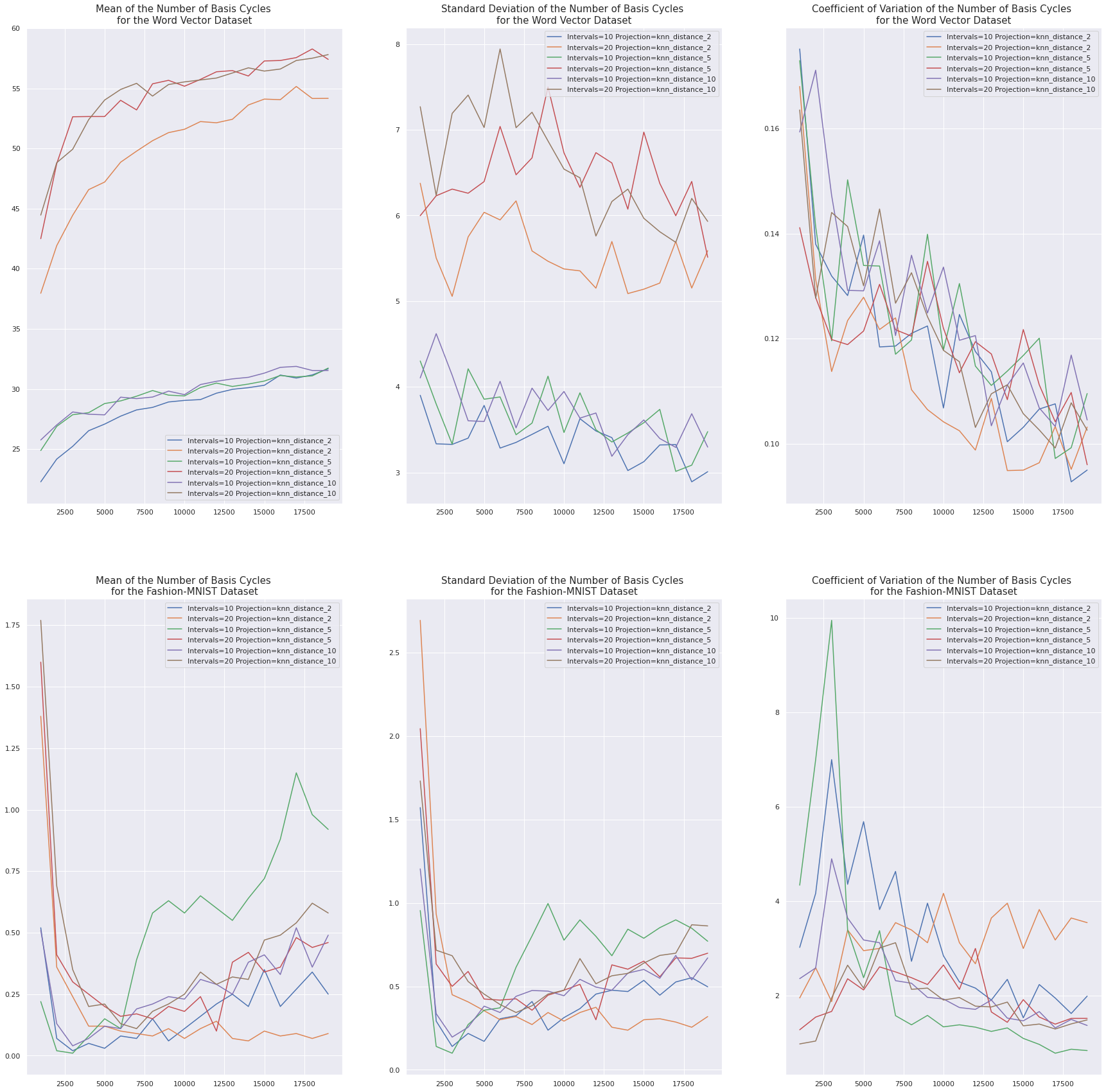
Cardinality of Cycle Basis
Word embeddings constructed with gloVe approximately satisfy an analogy property . If word A is to word B as word C is to word D, then \(v_{\text{B}} - v_{\text{A}}\) and \(v_{\text{D}} - v_{\text{C}}\) will be close in space. For example, we expect \(\|(v_{\text{king}} - v_{\text{queen}}) - (v_{\text{man}} - v_{\text{woman}})\|\) to be small. As a result of this property, there are long chains of related words in this dataset. This causes Mapper graphs formed from \(k\)-nearest neighbor projections over the Word Vector dataset to have many basis cycles. As we choose more samples from the Word Vector dataset the number of basis cycles tends to increase and stabilize, which causes this invariant’s coefficient of variation to decrease.
In contrast, the UMAP embeddings of the Fashion-MNIST dataset simply minimize the distance between points in the same class. As a result, Mapper graphs formed from \(k\)-nearest neighbor projections over the Fashion-MNIST dataset will have fewer than one basis cycle on average. Any cycles that do appear are probably noise, since there is no discernible decrease in the coefficient of variation of this graph invariant as the sample size increases.
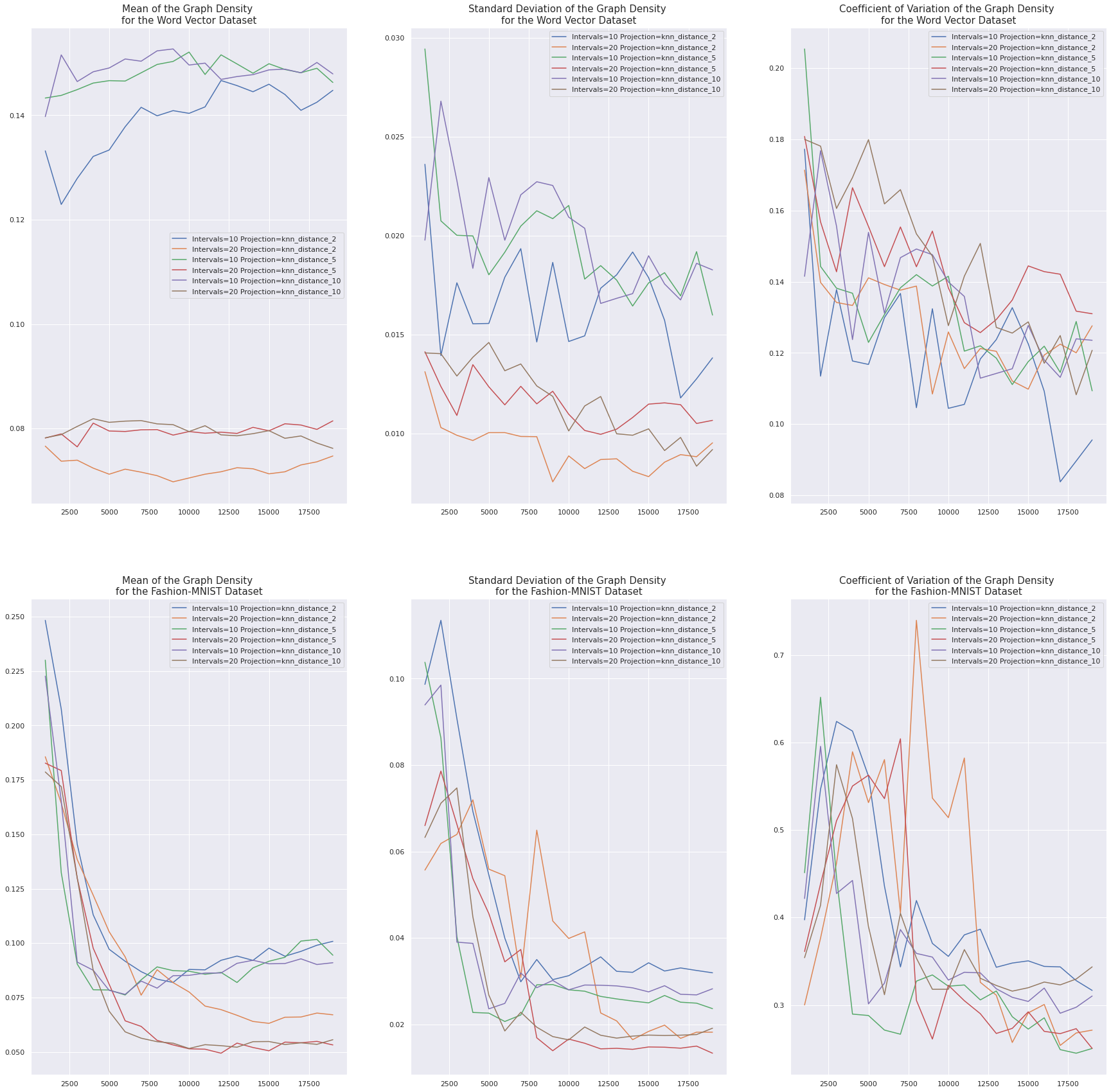
Graph Density
When the number of intervals is smaller we would expect the graph density to increase due to a smaller number of distinct clusters (fewer nodes) and more overlap between clusters (more edges). This effect is particularly pronounced in the Word Vector dataset, but it is also present for larger samples sizes in the Fashion-MNIST dataset.
In Fashion-MNIST the graph density tends to decrease as the number of samples increases, whereas it stays relatively constant in the Word Vector dataset. This is probably related to the separation of classes and the positive relationship between the sample size and the number of distinct connected components in Fashion-MNIST.
In both datasets the coefficient of variation of the graph density consistently decreases as the number of samples increases from \(10000\) to \(20000\), which suggests that these effects are not solely noise.
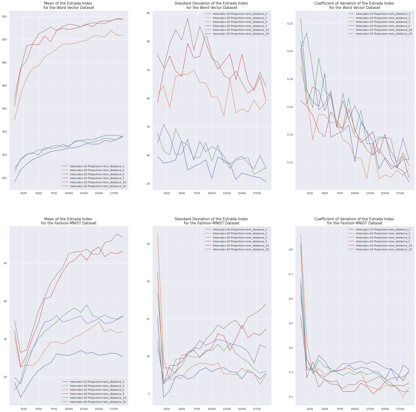
Estrada Index
When the number of intervals is smaller, we expect the smaller number of distinct clusters (fewer nodes) and more overlap between clusters (more edges) to cause each node to participate in a smaller proportion of subgraphs, which causes the Estrada index to decrease. This effect is particularly pronounced in the Word Vector dataset, but it is also present for larger samples sizes in the Fashion-MNIST dataset.
Furthermore, as the sample size increases we expect the sampled points to eventually cover the space, which should cause the centrality of the Mapper graph to converge. We see this in both datasets: the Estrada index tends to increase as the number of samples increases from \(0\) to \(10000\), and then level off. Furthermore, the coefficient of variation of the Estrada index tends to decrease as the number of samples increases.
General Observations
The mean values of all four metrics change very rapidly as the number of samples goes from \(1000\) to \(5000\) for Fashion-MNIST. This effect is much weaker for the Word Vector dataset, so this is probably caused by the need to sample enough images to reach a critical mass of representation across each of the \(9\) classes in this dataset.
Discussion
In this post we explore the relationship between the sample size and the stability of Mapper on two real-world datasets. We choose to focus on the \(k\)-nearest neighbor filter function, which is a non-parametric density estimator. In future work we aim to explore the stability of Mapper graphs formed from a wider class of filter functions, including other density estimators like the Gaussian kernel density estimator and other kinds of filters like the eigenfunctions of the covariance matrix. Furthermore, both of the datasets that we use in these experiments consist of embeddings learned with either gloVe or UMAP. These embedding algorithms have many hyperparameters, such as the dimensionality of the embeddings that are learned. In future work we will explore how the choice of these hyperparameters affects the noise sensitivity and stability of the Mapper output.
References
- Topological Methods for the Analysis of High Dimensional Data Sets and 3D Object Recognition
- Fashion-MNIST: a Novel Image Dataset for Benchmarking Machine Learning Algorithms
- GloVe: Global Vectors for Word Representation
- UMAP: Uniform manifold approximation and projection for dimension reduction
- Subgraph centrality in complex networks