Learning Complexity and Generalization Bounds

In a typical supervised learning setting, we are given access to a dataset of samples \(S = (X_1, y_1), (X_2, y_2), ..., (X_n, y_n)\) which we assume are drawn from a distribution \(\mathcal{D}\) over \(\textbf{X} \times \textbf{y}\). For simplicity, we will assume that \(\mathbf{X}\) is either the space \(\{0,1\}^n\) or \(\mathbb{R}^n\) and that \(\textbf{y}\) is either the space \(\{0,1\}\) or \(\mathbb{R}\).

Given a set of functions \(\mathcal{G}\) that map from \(\textbf{X} \rightarrow \textbf{y}\) and a loss function \(L\), the goal of supervised learning to find some \(g \in \mathcal{G}\) that minimizes \(E_{(X,y) \sim \mathcal{D}}[L(g(X), y)]\). For classification (when \(\textbf{y} = \{0,1\}\)), we commonly choose \(L\) to be the zero-one loss \(L(a,b) = \begin{cases} 0 & a=b \\ 1 & \text{else} \end{cases}\) . For regression (when \(\textbf{y} = \mathbb{R}\)), we often choose \(L\) to be the squared error \(L(a,b) = (a-b)^2\). Note that we could use the absolute error \(\vert a-b \vert\) instead of \((a-b)^2\), but squared error is differentiable everywhere and has a few other nice properties.

One significant challenge with this objective is that we generally cannot compute or optimize this expectation directly. Instead, we need to use the dataset \(S\) to estimate it. For example, we can use \(\frac{1}{n}\sum_{i=1}^{n} L(g(X_i), y_i)\) as an estimate of \(E_{(X,y) \sim \mathcal{D}}[L(g(X), y)]\). The quality of this estimate is dependent on a few factors:

• The number of samples \(n\)
• The choice of loss function \(L\). In this blog post we will primarily stick to the zero-one and squared error losses defined above
• The structure of the distribution \(\mathcal{D}\)
• The expressiveness of the function space \(\mathcal{G}\)

First, let’s consider the scenario when we fix a random element \(g \in \mathcal{G}\) and treat \(L(g(X), y)\) as a random variable on samples \((X,y) \sim \mathcal{D}\). Since the \((X_i,y_i)\) are drawn independently, we can treat \((L(g(X_1), y_1), L(g(X_2), y_2), ..., L(g(X_n), y_n))\) as a sequence of i.i.d random variables, and we can therefore apply the central limit theorem to bound the degree to which we expect \(\frac{1}{n}\sum_{i=1}^{n} L(g(X_i), y_i)\) to diverge from \(E_{(X,y) \sim \mathcal{D}}[L(g(X), y)]\). We refer to this kind of bound as a generalization bound.

In this case the magnitude of this divergence is determine by the variance of the random variable \(L(g(X), y)\). In addition to the number of samples \(n\), this variance is typically determined by the variance of the random variable \((X,y)\) itself, as well as the degree to which \(\mathcal{D}\) defines high-weight regions over \(\textbf{X} \times \textbf{y}\) that both agree with \(g\) and do not agree with \(g\).

Of course, in practice we do not fix \(g \in \mathcal{G}\) across different distributions \(\mathcal{D}\). Instead, we use some sort of optimization procedure to select \(g\) based on the samples \(S\) that we have drawn from \(\mathcal{D}\). In this situation we will need to formulate generalization bounds that depend on \(\mathcal{G}\) directly.

Polynomial Example

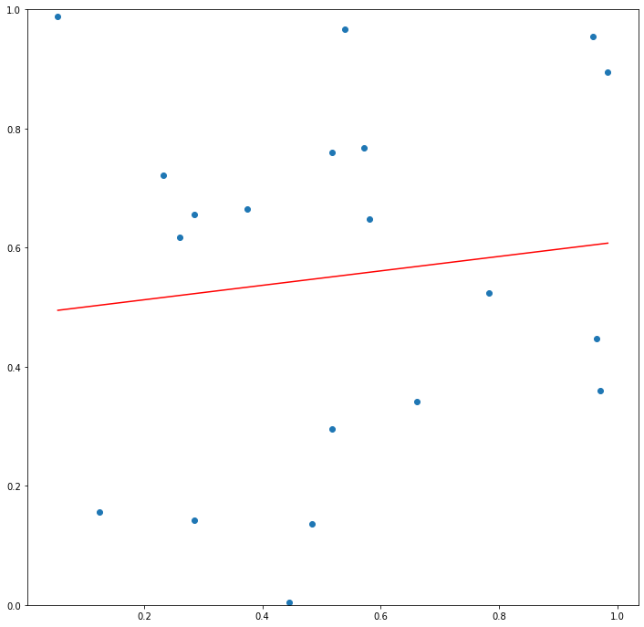
Let’s start by considering a simple regression example. Say that both \(\mathbf{X}\) and \(\mathbf{y}\) are \(\mathbb{R}\) and that \(\mathcal{D}\) is a completely uniform distribution over the interval \([0,R] \times [0,R]\) such that there is no relationship between \(\mathbf{X}\) and \(\mathbf{y}\). Obviously, we would expect that for any function \(g\), \(E_{(X,y) \sim \mathcal{D}}[L(g(X), y)]\) will be consistently well above \(0\) and will increase with \(R\).

Now let’s say that \(\mathcal{L}\) is the class of linear functions such that we can express any \(g\in\mathcal{L}\) as \(g(x) = a*x + b\). If \(n=2\), we can always draw a line that connects the two points and have \(L(g(X_1), y_1) + L(g(X_2), y_2) = 0\). However, for large \(n\), it is likely that no line will come close to connecting the points, and for any \(g \in \mathcal{L}\) the quantity \(\frac{1}{n}\sum_{i=1}^{n} L(g(X_i), y_i)\) will be close to \(E_{(X,y) \sim \mathcal{D}}[L(g(X), y)]\).

Now say that we instead define \(\mathcal{P}\) to be the class of polynomials. Since for any set of \(n+1\) points in the plane with distinct \(X\) and \(y\) values there always exists a degree \(n\) polynomial that passes through those points, there will always exist some \(g \in \mathcal{P}\) such that \(\frac{1}{n}\sum_{i=1}^{n} L(g(X_i), y_i)\) will be \(0\).

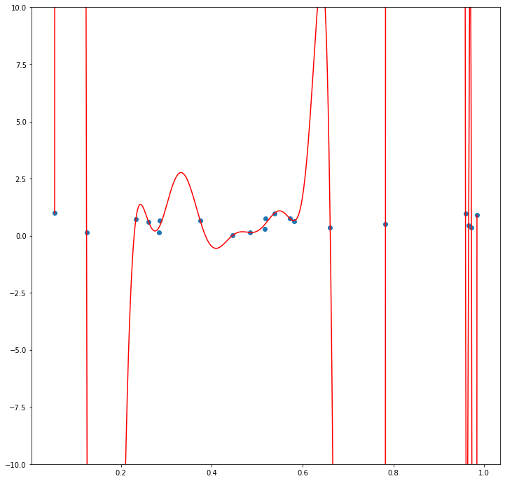
Intuitively, we can see that for this “worst case” distribution, a larger and more complex function class will exhibit a greater difference between \(\frac{1}{n}\sum_{i=1}^{n} L(g(X_i), y_i)\) for the \(g \in \mathcal{G}\) that minimizes this value and \(E_{(X,y) \sim \mathcal{D}}[L(g(X), y)]\) for this same \(g\). The reason for this is that for any particular realization of “noise” \(S = (X_1, y_1), (X_2, y_2), ..., (X_n, y_n)\), a larger and more complex function class has a higher probability of containing some function \(g\) that can “fit” that noise.

Rademacher Complexity

We can make this rigorous. The Rademacher Complexity of a function class \(\mathcal{G}\) over a distribution \(\mathcal{D}_X\) measures the degree to which the outputs of a function \(g \in \mathcal{G}\) on \(X_1, X_2, ..., X_n \sim \mathcal{D}_X\) can correlate with a sequence of i.i.d random variables \(\sigma_1, \sigma_2, ..., \sigma_n\) that are uniformly distributed on \([-1,1]\) (i.e. Rademacher random variables). That is:

Unsurprisingly, the larger the Rademacher complexity of a function class \(\mathcal{G}\), the greater the divergence between \(\frac{1}{n}\sum_{i=1}^{n} g(X_i)\) for the \(g \in \mathcal{G}\) that minimizes this value and \(E_{X \sim \mathcal{D}_X}[g(X)]\) for this same \(g\). If we compute the Rademacher complexity of the function class \(\mathcal{G}^L = \{(X,y) \rightarrow L(g(X), y\ \vert\ g \in \mathcal{G}\}\) from the Rademacher complexity of \(\mathcal{G}\), we can use this property to bound the divergence between \(\frac{1}{n}\sum_{i=1}^{n} L(g(X_i), y_i)\) for the \(g \in \mathcal{G}\) that minimizes this value and \(E_{(X,y) \sim \mathcal{D}}[L(g(X), y)]\) for this same \(g\). Let’s note that by Talagrand’s lemma the Rademacher complexity of \(\mathcal{G}^L\) depends on \(L\) as well as \(\mathcal{G}\), and can be significantly larger than \(\mathcal{G}\) for faster growing loss functions (e.g. \(L(a,b) = (a-b)^k\) for large \(k\)).

VC Dimension

One of the major downsides of Rademacher complexity is that it is distribution-dependent. That is, the Rademacher complexity of a function class \(\mathcal{G}\) is defined with respect to the marginal distribution \(\mathcal{D}_X\) over \(\textbf{X}\). However, in practice we may not have access to this distribution, and it could be useful to reason about how the function class \(\mathcal{G}\) will behave over the worst case distribution.

One tool for doing this is VC Dimension, or Vapnik-Chervonenkis Dimension. Unlike Rademacher Complexity, VC Dimension is only defined for classification. That is, we can only compute the VC dimension of function classes that map into \(\{0, 1\}\). Both the Rademacher Complexity and VC dimension of a function class measure the expressiveness of the class, or the degree to which the “best” function in the class can generate outputs that are consistent with somewhat arbitrary (input, output) pairs. However, unlike Rademacher Complexity, VC dimension does not measure this expressiveness probabilistically.

We define the VC dimension of a function class \(\mathcal{G}\) to be the largest set of points \((X_1, X_2, ...)\) that the function class can shatter, or classify in every possible way. For example, consider the class \(\mathcal{G}\) of interval functions on \(\mathbb{R} \rightarrow \mathbb{R}\). That is, the class of functions that we can express as \(g_{a,b}(X) = \begin{cases} 1 & a<=X<=b \\ 0 & \text{else} \end{cases}\) . For the set of two points \((X_1, X_2) = (1, 2)\), there exists four possible labelings of that set:

\((y_1, y_2) = (0,0)\), \((y_1, y_2) = (0,1)\), \((y_1, y_2) = (1,0)\) and \((y_1, y_2) = (0,0)\)

For each of these labelings, we can define an interval that contains all points labelled \(1\) and no points labelled \(0\). However, for any set of three distinct points \((X_1, X_2, X_3)\) ordered from smallest to largest, there exists no interval function that can generate the classification \((1,0,1)\). Therefore, the VC dimension of \(\mathcal{G}\) is \(2\).

Intuitively, if the VC dimension of \(\mathcal{G}\) is very large, then even when \(n\) is large it is possible for a learning algorithm to find a \(g \in \mathcal{G}\) that has a very low sample loss \(\frac{1}{n}\sum_{i=1}^{n} L(g(X_i), y_i)\) even when \(\mathbf{X}\) and \(\mathbf{y}\) are independent over \(\mathcal{D}\). That is, it is possible for \(E_{(X,y) \sim \mathcal{D}}[L(g(X), y)]\) and \(\frac{1}{n}\sum_{i=1}^{n} L(g(X_i), y_i)\) to be very different.

One important aspect of VC dimension is that \(\mathcal{G}\) only needs to be able to shatter one set of size \(d\) in order to have a VC dimension of \(d\). This is a consequence of the “worst case” focus of VC dimension. In order to make claims that are distribution-agnostic, we need to focus on how a learning algorithm for \(\mathcal{G}\) performs even when the distribution \(\mathcal{D}\) is chosen adversarially.

As a consequence of this, there are many function classes that have very high or even infinite VC dimension, but have more managable Rademacher Complexity if we make even mild assumptions about \(\mathcal{D}_X\) (see the k-split interval classifiers in this paper for an example).

Occam’s Razor

One thing to note about both Rademacher Complexity and VC dimension is that they tend to be correlated with the minimum number of bits we would need to uniquely identify a member of the corresponding function class. For example, consider the function class \(\mathcal{P}^d\) of \(0,1\)-coefficient polynomials of degree \(d\). As \(d\) increases, the VC dimension, Rademacher complexity, and number of bits required to uniquely identify each polynomial increases. This is a consequence of a much more general principle known as Occam’s Razor, which roughly states that simpler explanations tend to be more robust than complex explanations. There are deep information theoretic arguments for why this is the case, see this paper for more information.

Regularization

In most modern Machine Learning applications, researchers work with extraordinarily complex function classes, such as deep neural networks or massive forests of decision trees. These function classes have extremely high or even infinite VC dimension and Rademacher Complexity. However, modern learning algorithms are capable of finding functions whose performance generalizes well regardless. One reason for this is the prevalence of regularization techniques, which guide learning algorithms towards lower complexity subregions of high complexity function spaces.

For example, consider the class \(\mathcal{L}^W\) of linear functions such that the weight vector \(w\) of the model has norm \(\|w\| \leq W\). The Rademacher Complexity of this class increases with \(W\). In general, the most popular algorithms for learning the values of these weights use gradient based methods for minimizing the loss function \(\frac{1}{n}\sum_{i=1}^{n} L(g(X_i), y_i)\) that do not explicitly restrict their search space to vectors with small norm. However, it is quite common to add a regularization term and use the algorithm to minimize the loss function \(\|w\| + \frac{1}{n}\sum_{i=1}^{n} L(g(X_i), y_i)\) instead. That is, although a learning algorithm may be searching the high Rademacher complexity function space \(\mathcal{L}^\infty\), the optimization criteria incentivizes the algorithm to prefer solutions in the low Rademacher Complexity region of linear classifiers with small \(\|w\|\).

Resources

Most of the content in this post is from An Introduction to Computational Learning Theory by Michael J. Kearns, as well as the “Learning Real Valued Functions” and “VC dimension” course notes from Varun Kanade’s Computational Learning Theory course at Oxford.