Representing Graphs with Low Dimensional Matrix Factorization for Fun and Profit

A solid laptop computer in 2018 has about 1TB (1000GB) of disk space, and the capability to store about 16GB of memory in RAM. In comparison, internet users in the United States generate about 3000TB of data every minute ¹. An enormous amount of this data takes the form of high dimensional sparse relationships that are difficult to efficiently model.

In order to effectively harness and interpret this data, researchers and organizations have relied heavily on algorithms like neural networks that work best on low dimensional dense data. In this article I will describe one technique for reducing large high dimensional sparse data to small low dimensional dense data that is compatible with machine learning algorithms like neural networks.

Representing Graphs

Say we have a set of entities (words, people, movies, etc) and we want to represent some relation between them. For simplicity’s sake, let’s say that we are interested in a binary relation, such as “these two people are friends”, or “these two movies have a shared co-star.” We can represent these entities and this relation in an unweighted graph \(G\) in which we represent each entity with a node and the relation with the edges between the nodes.

One common way of storing \(G\) is an adjacency matrix - i.e. an \(NxN\) matrix \(A\), where \(N\) is the number of nodes and entry \(A_{ij}\) is \(1\) if an edge exists between nodes \(N_{i}, N_{j}\) and \(0\) otherwise. However, since this matrix is typically extremely large and sparse, it can be prohibitive to store and manipulate for very large graphs. One way to avoid this is to instead use a low-rank symmetric matrix factorization algorithm to form the \(NxD\) matrix \(V\), where \(VV^{T}\) is an approximation of \(A\). Intuitively, we are assiging to each node \(N_i\) in \(G\) a \(D\) dimensional vector \(V_i\) such that for any two nodes \(N_i, N_j\) in \(G\), the dot product \(V_{i}V_{j}^{T}\) is indicative of the likelihood that an edge exists between \(N_{i}\) and \(N_{j}\). This can allow us to represent our entities and their relationships in much less space. Furthermore, the low dimensional entity representations are often easier to use in Machine Learning tasks than the sparse high dimensional graph representations.

Now consider the case where the relationship between entities is no longer binary, for example, the relationship between two movies might be their number of shared actors. In this case:

• \(G\) becomes a graph with weighted edges.
• \(A_{ij}\) is \(x\) if an edge with weight \(x\) exists between nodes \(N_{i}, N_{j}\) and \(0\) otherwise.
• The dot product \(V_{i}V_{j}^{T}\) is as close as possible to \(x\).

In some cases, the continuous graph might be quite dense. Consider the case where our entities are the words in the English language and the relationship between words is the frequency with which they appear together in a sentence, perhaps normalized by their individual frequencies (PMI). In this case \(A\) is a large, dense matrix that’s likely impossible to store in memory and factorize directly. We could instead apply an algorithm like the following to symmetrically factorize it:

• Randomly initialize the \(nxd\) matrices \(W\)
• For each tuple \(w_i,w_j,x\) where \(x\) is the number of times that \(w_i\) and \(w_j\) appear in a sentence, take a gradient descent step towards minimizing the loss \(\|x - W_{i}^{T}W_{j}\|\).

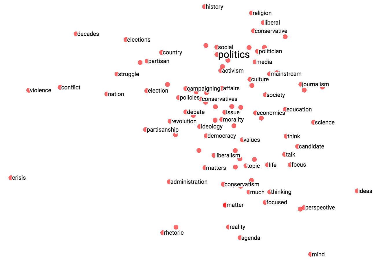
This will produce “word embeddings” for each word in our vocabulary such that the dot product between any two word’s embeddings is indicative of the frequency with which the words appear in a sentence. Note that if we use an additional matrix to represent word context and modify the loss function a bit, we get the skigram algorithm from Mikolov’s word2vec. In the image below, we demonstrate how similar words appear closer to each other in the word vector space:

Representing Bi-Partite Graphs

Now consider the case where we instead want to represent the affinities between a group of entities of type 1 and a group of entities of type 2. For example, we may want to represent the rating a user would give to a movie or the likelihood that a user would click on an advertisement.

We can represent these relationships with a bi-partite graph \(B\) where the two disjoint sets of nodes correspond to the two types of entities. You can see an example for users and movies below:

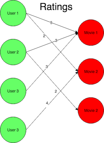
We can use a modified adjacency matrix \(A_{B}\) to represent \(B\). Say we have \(N\) entities of type \(E_1\) and \(M\) entities of type \(E_2\). Then define \(A_{B}\) to be the \(NxM\) matrix such that entry \(i,j\) of \(A_{B}\) is equal to the weight of the connection between entity \(i\) of type \(E_1\) and entity \(j\) of type \(E_2\). We can use a technique similar to those described above to represent \(B\) with two matrices of low dimensional entity vectors.

For example, if we take the reduced SVD of \(A_{B}\) with dimension \(D\), we get the orthogonal \(NxD\) matrix \(U\), the orthogonal \(MxD\) matrix \(V\) and the diagonal \(DxD\) matrix \(S\) such that \(\|A_B - USV^{T}\|\) is minimized. We can “absorb” \(S\) into \(U\) and \(V\) to form \(U^{*}=US^{1/2}\) and \(V^{*}=VS^{1/2}\) such that \(\|A_B - U^{*}V^{*T}\|\) is still minimized.

Note that each row \(U_i^{*}\) of \(U^{*}\) corresponds to entity \(i\) of type \(E_1\) and each row \(V_j^{*}\) of \(V^{*}\) corresponds to entity \(j\) of type \(E_2\) such that the affinity between entity \(i\) and entity \(j\) is correlated to \(U_i^{*}V_j^{*}\). Note that this is equivalent to constructing a linear regression model for each entity \(j\) of type \(E_2\) and projecting each entity \(i\) into a space such that the outputs of each \(j\)’s linear regression model on \(i\)’s projection is an estimate of the affinity between entity \(i\) and entity \(j\). We refer to this as a “co-embedding” between the entity types \(E_1\) and \(E_2\).

Conclusion

We can represent most entity relationships with graphs. However, large sparse graphs are difficult to store and query. Furthermore, node-edge relationships are difficult to utilize as features for machine learning algorithms. Matrix factorization approaches can efficiently model and represent the nodes of these graphs with low dimensional vectors.